Combining principles; Theorem 3

When each of the \( M \) branch networks and source resistances are identical there is an equivalence between the multiport combiner with source resistance below and the single branch network also shown below, comprised of an effective source resistance \( R_{e} \), a scaled branch network \( \mathbf{Y_{e}} \) and the original trunk network \( \mathbf{Z_{t}} \).

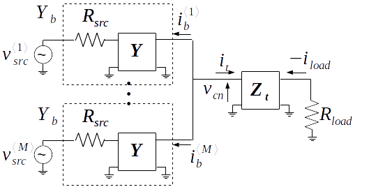
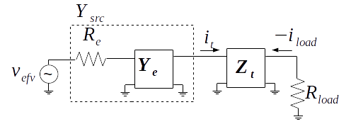
Theorem 3. When each of the \( M \) branch networks and source resistances are identical there is an equivalence between the multiport combiner with source resistance above and the single branch network also shown above, comprised of an effective source resistance \( R_{e} \), a scaled branch network \( \mathbf{Y_{e}} \) and the original trunk network \( \mathbf{Z_{t}} \) such that

\begin{equation} \label{eq:refv} R_{e} = \frac{R_{src}}{M} \end{equation}

and

\begin{equation} \label{eq:yefv} \mathbf{Y_{e}} = M \mathbf{Y} \end{equation}

Proof. Assume that (\ref{eq:refv}) and (\ref{eq:yefv}) are true. Using the conventional formulae for conversion between admittance and cascade parameters ¹, or standard charts on a Grassmanian manifold ² the effective source resistance is cascaded with the effective admittance network in each branch.

\begin{equation} \label{eq:ysrcdef} \mathbf{Y_{src}} = \left[ \begin{array}{cc} \frac{M Y_{e_{11}}}{R_{e} Y_{e_{11}} + 1}& \frac{M Y_{e_{12}}}{R_{e} Y_{e_{11}} + 1} \\
\frac{M Y_{e_{21}}}{R_{e} Y_{e_{11}} + 1}& \frac{M \left( R_{e} (Y_{e_{11}} Y_{e_{22}} - Y_{e_{12}} Y_{e_{21}}) + Y_{e_{22}} \right) }{R_{e} Y_{e_{11}} + 1} \\
\end{array} \right] \end{equation}

From Theorem 2 it is known that when all the branches are identical multiple sources driving the combiner are equivalent to a single source that is the sum of the multiple sources. In this case the branch admittances of the above ideal combiner circuit are in parallel and as a result

\begin{equation} \label{eq:ytotaldef} \mathbf{Y_{total}} = M \mathbf{Y_{b}} \end{equation}

\( \mathbf{Y_{b}} \) is the cascade of \( R_{src} \) and \( \mathbf{Y} \) which results in

\begin{equation} \label{eq:ybdef} \mathbf{Y_{b}} = \left[ \begin{array}{cc} \frac{Y_{11}}{R_{src} Y_{11} + 1}& \frac{Y_{12}}{R_{src} Y_{11} + 1} \\
\frac{Y_{21}}{R_{src} Y_{11} + 1}& \frac{R_{src} (Y_{11} Y_{22} - Y_{12} Y_{21}) + Y_{22}}{R_{src} Y_{11} + 1} \\
\end{array} \right] \end{equation}

and finally, from (\ref{eq:ysrcdef}), (\ref{eq:ytotaldef}) and (\ref{eq:ybdef})

\begin{equation} \mathbf{Y_{src}} = M \mathbf{Y_{b}} \end{equation}

Corollary. The effective source resistance \( R_{e} \) is given by (\ref{eq:refv}) iff the circuits in each branch and the source resistances of each branch are identical.