A combining network driven by multiple voltage sources as shown in the figure of Theorem 1 is equivalent to the same network driven by a single voltage source as shown below.
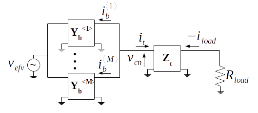
Theorem 2. A combining network driven by multiple voltage sources as shown in the figure of Theorem 1 is equivalent to the same network driven by a single voltage source as shown above when
\begin{equation} \label{eq:vefv} v_{efv} = \sum_{k = 1}^{M} v^{\langle k \rangle}_{src} \end{equation}
and all the branch admittances are identical
\begin{equation} \mathbf{Y_{b}} = \mathbf{Y}_{b}^{\langle 1 \rangle} = … = \mathbf{Y}_{b}^{\langle k \rangle} = … = \mathbf{Y}_{b}^{\langle M \rangle} \end{equation}
Proof. Using the same method for solving for the load voltage \( v_{load} \) as in Theorem 1 the load voltage of the network of the above single source equivalent network is
\begin{equation} v_{load} = a_{outer} v_{efv} \sum_{k = 1}^{M} a^{\langle k \rangle}_{inner} \end{equation}
If all the branch admittances are identical and \( v_{efv} \) is defined as (\ref{eq:vefv}), then
\begin{equation} \label{eq:equivsrc} v_{load} = a_{outer} M Y_{b_{21}} \sum_{k = 1}^{M} v^{\langle k \rangle}_{src} \end{equation}
and (\ref{eq:equivsrc}) is equivalent to the \( v_{load} \) equation from Theorem 1 when the branch admittances are the same.
Corollary. The proof for current source drive is equivalent to the above by making the H-parameter substitutions from the Corollary to Theorem 1 and
\begin{equation} v_{efv} = i_{efv} \end{equation}
into (\ref{eq:equivsrc}).