This tutorial gives an overview of multiport black-box model theory and how it relates to commonly used parameters of linear, time invariant electrical networks. Expressions are also derived for the conversions between the various multiport parameters.
Multiport black box models
The theory presented here is derived from a paper by Pauli1 which identifies the correspondence between abstract geometric concepts and black-box models used to model physical systems.
A multiport black-box model describes a physical system in terms of the behaviour of parameters defined exclusively at the terminals of the model. In circuit networks these parameterisations are usually in the frequency domain although they may also be used under specific conditions in the time domain.
For every port there are two terminals and thus an N-port model has \( 2 N \) terminals. Each port is described by two coordinates as shown below.
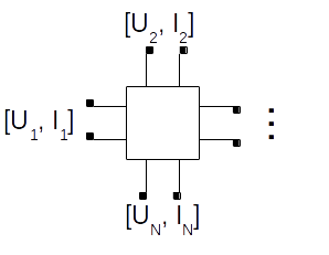
In a circuit network the coordinates may be potential and current, or incident and reflected waves (although Kurokawa2 alludes to the fact that other choices of coordinates are available, they have not been defined). These coordinates form an orthogonal basis \( B \) on a noncompact Stiefel manifold as shown in equation \ref{eq:gen-basis}.
\begin{equation}
B = \left[
\begin{array}{c}
U \\
I
\end{array}
\right]
\label{eq:gen-basis}
\end{equation}
The various parameters of a multiport network are charts on the manifold. In
general there are \( \left(
\begin{array}{c}
2 N \\
N
\end{array}
\right) \) charts that may be determined corresponding to the parameters
available for a given number of ports. Thus, for example, for two-port networks
there are six charts (that is, six different types of parameters) and for
three-port networks there are twenty charts.
Systematic identification of parameter transforms
The six charts for two-port networks in the \( [i, v] \) (current and voltage) domain are well known 3. They are commonly referred to as Z-, Y-, H-, G-, Cascade1- and Cascade2- parameters. The problem is that \( \frac{2}{3} \) of these parameters do not extend to multiport networks. Thus some method is needed to systematically identify multiport parameters and the transformations between them.
A notation is introduced here for systematically identifying the transformations between parameters.
Conversions within the \( [i, v] \) parameter domain
Consider the state equation for Z-parameters
\[ 1_{N} v = Z i \]
Expressing this in terms of the basis
\begin{equation}
B = \left[
\begin{array}{c}
v_{1} \\
\vdots \\
v_{N} \\
i_{1} \\
\vdots \\
i_{N}
\end{array} \right]
= \left[
\begin{array}{c}
Z \\\ 1_{N}
\end{array} \right] i
= \left[
\begin{array}{c}
1_{N} \\\ Y
\end{array} \right] v
\end{equation}
\begin{equation} \left[ \begin{array}{c} Z \\\ 1_{N} \end{array} \right] \left[ Z \right]^{-1} = \left[ \begin{array}{c} 1_{N} \\\ Y \end{array} \right] \end{equation}
Conversions within the \( [a, b] \) parameter domain
It is worth observing that using the differentiable manifold theory it becomes apparent that for 2-port scattering parameters there are in fact six possible parameters analogous to the familiar 2-port parameters in the \( [i, v] \) domain. Two of these correspond to the forward and reverse cascade forms, sometimes described as forward and reverse transmission parameters, or T-parameters. If the S-parameters are considered analogous to the Z-parameters coordinates in the sense that \( v \) is a function of \( Z \) and \( i \) in the same way that \( b \) is a function of \( S \) and \( a \) then there must logically be another parameter that is analogous to the Y-parameters in the sense that \( a \) is a function of \( R \) and \( b \).
\[ a = R b \]
Conversion between \( [a, b] \) and \( [i, v] \) parameter domains
RF designers are familiar with the relations converting a reflection coefficient (S11 in a single port system) to impedances 4, or an impedance back to reflection coefficient 5. The problem with these common relations is that they are only valid for a single port system or a two port system by making certain assumptions about the load termination. There are tables of formulae in some tutorials 6 supposedly giving a conversion between two port S-parameters and Z- or Y- parameters but these formulations are often incorrect because they fail to take into account that the S-parameters are referred to a specific non-infinite and non-zero load impedance, but Z- and Y- parameters are referred respectively to infinite and zero load impedances. By returning to the original S-parameter definitions by Kurokawa 2 and taking some care to preserve the noncommutative properties of the matrix expressions then relatively simple expressions valid for an arbitrary number of ports may be derived.
The \( [a, b] \) parameters that define S-parameters are fundamentally related to the \( [i, v] \) parameters by the expressions originally derived by Kurokawa. The expressions are restated here in matrix form which emphasises the noncommutative properties used to combine the various column vector parameters.
\begin{equation} a = \frac{1}{2} \left[ K \right] ^{-1} ( v + Z_{p} i ) \label{eq:adfn} \end{equation}
\begin{equation} b = \frac{1}{2} \left[ K \right] ^{-1} ( v - Z_{p}^{*} i ) \label{eq:bdfn} \end{equation}
Where \( i \) and \( v \) are the respective column vectors of current and voltage at each port and \( Z_{p} \) is the diagonal matrix of the complex termination impedances for each port. Finally,
\[ K = \sqrt{\left| \Re (Z_{p}) \right|} \]
Note that when \( Z_{p} \) are complex impedances the equations \ref{eq:adfn} and \ref{eq:bdfn} are implicitly in the frequency domain. If \( Z_{p} \) are purely resistive (real) then the equations may be either time or frequency domain due to linearity.
Converting between S and Y parameters
The respective terminal equations for S and Y parameters are
\[
\begin{array}{c}
b = S a
i = Y v
\end{array}
\]
Substituting the expressions for \( a \), \( b \) and \( i \)
\[ \left[ K \right]^{-1} v - \left[ K \right]^{-1} Z_{p}^{*} Y v = S \left( \left[ K \right]^{-1} v + \left[ K \right]^{-1} Z_{p} Y v \right) \]
The \( v \) terms cancel, leaving
\[ \left[ K \right]^{-1} - \left[ K \right]^{-1} Z_{p}^{*} Y = S \left[ K \right]^{-1} + S \left[ K \right]^{-1} Z_{p} Y \]
Solving for Y in terms of S yields
\begin{equation} Y = \left[ S \left[ K \right]^{-1} Z_{p} + \left[ K \right]^{-1} Z_{p}^{*} \right] ^{-1} (1_{N} - S) \left[ K \right]^{-1} \end{equation}
Solving for S in terms of Y yields
\begin{equation} S = \left[ K \right] ^{-1} (1_{N} - Z_{p}^{*} Y) \left[ 1_{N} + Z_{p} Y \right] ^{-1} K \end{equation}
Converting between S and Z parameters
Starting with the terminal equations for S and Z parameters
\[ v = Z i \]
Substituting the expressions for \( a \), \( b \) and \( v \)
\[ \left[ K \right] ^{-1} Z i - \left[ K \right] ^{-1} Z_{p}^{*} i = S \left( \left[ K \right] ^{-1} Z i + \left[ K \right] ^{-1} Z_{p} i \right) \]
The \( i \) terms cancel, leaving
\[ \left[ K \right] ^{-1} Z - \left[ K \right] ^{-1} Z_{p}^{*} = S \left[ K \right] ^{-1} Z + S \left[ K \right] ^{-1} Z_{p} \]
Solving for Z in terms of S yields
\begin{equation} Z = K \left[ 1_{N} - S \right] ^{-1} \left( S \left[ K \right] ^{-1} Z_{p} + \left[ K \right] ^{-1} Z_{p}^{*} \right) \end{equation}
Solving for S in terms of Z yields
\begin{equation} S = \left[ K \right] ^{-1} (Z - Z_{p}^{*}) \left[ Z + Z_{p} \right] ^{-1} K \end{equation}
List of Symbols
| \( \left( \begin{array}{c} n \\\ k \end{array} \right) \) | Combinations of ( k ) in ( n ) |
| \( \Re (z) \) | Real part of complex number \( z \) |
| \( \left[ \right] ^{-1} \) | Matrix inverse |
| \( z^{*} \) | Complex conjugate of \( z \) |
| \( 1_{N} \) | \( N \times N \) identity matrix |
-
Differentiable manifolds and engineering black-box models for linear physical systems, Rainier Pauli, Proc. Int. Symp. Mathematical Theory of Networks and Systems (MTNS), Perpignan, France, 2000. ↩
-
Power waves and the scattering matrix, K. Kurokawa, IEEE Trans. Micr. Theory \& Tech., 1965, pp194-202 ↩ ↩2
-
Electric Circuits, Nilsson, Prentice Hall, 1993 ↩
-
S-parameters, circuit analysis and design, Hewlett-Packard Application Note 95 (Keysight Technologies). ↩
-
S-parameter design, Agilent Technologies Application Note 154. ↩
-
S-parameter techniques for faster, more accurate network design, Hewlett-Packard Application Note 95-1 (Keysight Technologies). ↩